
Summary
This proposal suggests the PI Controller and Collateral Factor parameters and outlines the quantitative methodology used to arrive at these values.
Problem definition
Open Dollar is a stablecoin protocol that permits users to borrow the stable $OD against a predefined set of collateral assets. To maintain its peg, the protocol employs a PI Controller to dynamically adjust the redemption rate, influencing the redemption price of the issued stablecoin. This mechanism creates arbitrage opportunities that help align the market price of $OD with the target price of $1. Moreover, each collateral asset is assigned a Collateral Factor to safeguard the system against insolvency during market fluctuations.
The design of the protocol leads to two primary questions:
- What are the PI Controller settings to ensure that $OD remains soft-pegged to $1?
- What should the initial Collateral Factor be for each asset at the launch of the protocol?
Methodology
Agent-based Modeling
Agent-based modeling (ABM) is a sophisticated simulation technique that is particularly well-suited for analyzing complex systems such as decentralized finance (DeFi) protocols. In contrast to traditional models that predict outcomes based on aggregate behaviors, ABM focuses on simulating individual agents. Each agent is modeled with distinct decision-making strategies and access to information, allowing them to interact within the marketplace independently. This approach is highly effective at capturing the varied behaviors and interactions within DeFi ecosystems, where the actions of numerous participants significantly influence overall dynamics. Utilizing ABM can uncover emergent patterns and potential nonlinear effects, providing essential insights into the resilience and potential vulnerabilities of systems like Open Dollar.
Open Dollar Implementation
Protocol Initialization
Our simulation engine is designed to replicate the fundamental mechanics of the Open Dollar system. Each simulation operates over a 30-day period, with time advancing in one-hour increments. We incorporate historical price data for the collateral assets as input variables. For each simulation cycle, a new set of 30-day historical price data is randomly selected.
At the start of the simulation, user positions within the protocol are generated randomly. The maximum Loan-to-Value (LTV) ratio for any user is capped by the collateral factors assigned to their respective assets. To ensure realism and maintain scalability in our model, we adjust the size of user positions so that the total amount of $OD borrowed aligns with what might be expected for a newly launched protocol. The accompanying chart illustrates an example distribution of user portfolios.
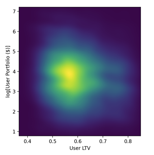
Figure 1.: User portfolio distributions at the initialization of Open Dollar simulation
Agent Behavior
During each time step of our simulation, users have the option to either mint new $OD by opening new positions or redeem some of their collateral by repaying portions of their debt. To simulate these activities, we employ a stochastic model that uses a Poisson process. This choice is particularly apt as the Poisson process is excellent for modeling the likelihood of a certain number of events occurring within a predefined time period, effectively capturing the random timing of user actions in the protocol.
Additionally, we implement a sampling technique to realistically model the magnitude of minting or redeeming actions. This involves drawing from a predetermined distribution that accurately reflects the range of transaction sizes observed within the system.
The probability distributions used to govern these processes are derived from empirical data collected from another stablecoin project, Liquity. The chart below shows the data from Liquity’s minting and redeeming activities and the corresponding probability distribution that we have calibrated for use in our simulations.

Figure 2.: Daily mint and burn distributions in Liquity with Weibull probability distribution fit
Within our simulation, agents can also engage in arbitrage, which presents itself under two specific conditions:
- Arbitrage Opportunity when Redemption Price Exceeds Market Price
If the redemption price of $OD is higher than its market price, users are motivated to buy $OD on the secondary market (for example, through a decentralized exchange or DEX) and use it to redeem a portion of their collateral. This action not only results in a profit for the users due to the price differential but also exerts an upward pressure on the market price of $OD. - Arbitrage Opportunity when Market Price Exceeds Redemption Price
Conversely, if the $OD redemption price is lower than the market price, users are encouraged to mint new $OD by depositing collateral into the system and then converting their newly minted $OD back into collateral assets on a secondary market. This increases the overall size of the protocol, allows users to realize a profit, and tends to decrease the market price of $OD. However, for this arbitrage to be viable, the price difference must exceed the complement of the Loan-to-Value (1-LTV) ratio for the collateral asset involved. Consequently, this form of arbitrage is triggered less frequently.
Liquidations
At each time step, the open user positions get updated by the new asset prices sampled from the historical data. Occasionally, these updates may lead to liquidations if the Loan-to-Value (LTV) ratio of a user’s position exceeds the maximum allowed by their collateral assets.
In the Open Dollar system, any vault eligible for liquidation is directed to an auction house. Here, market participants can place bids to acquire the underlying collateral. Effectively, each liquidation can have a different liquidation incentive. Commonly, liquidators convert the repossessed collateral into the debt asset immediately, avoiding a speculative position on the collateral asset. This conversion may cause a price impact which, in turn, affects the profitability of the liquidation. Liquidators will only proceed with liquidation if it is profitable — otherwise, they abstain, as non-profitable liquidations do not incentivize their participation.
The dynamics of liquidation have significant implications for the financial stability of the protocol. If the liquidation incentive is excessively high compared to the LTV of the liquidated user, the protocol risks accumulating bad debt (see more). Conversely, if the price impact incurred by liquidators when exiting the collateral is substantial, potential liquidations may not occur. This scenario can leave the protocol vulnerable to positions that might soon escalate into bad debt.
Our simulation engine meticulously incorporates these liquidation mechanics. We use a probability distribution for liquidation incentives based on empirical data from Euler V1, which implemented an auction-based liquidation model. The distribution used in our simulations is illustrated in the chart below, offering a detailed view of potential outcomes and their frequencies.
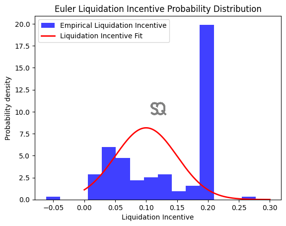
Figure 3.: Realized Liquidation incentive sampled from Euler V1 with a probability distribution fit
PI Controller
Central to the Open Dollar system is the PI Controller, which is designed to stabilize the $OD price at $1 by adjusting the redemption rate. This mechanism works as follows:
- When the market price of $OD exceeds the redemption price, the PI Controller reduces the redemption rate, which in turn lowers the redemption price to align closer to the market price.
- Conversely, if the market price is below the redemption price, the PI Controller increases the redemption rate, thereby raising the redemption price to meet the market level.
Our simulation engine encapsulates this regulatory mechanism. Alongside the arbitrage opportunities that it enables, the PI Controller plays a crucial role in maintaining the market price at $1, provided the hyperparameters are optimally set. The effectiveness of the PI Controller can be observed in the chart below, where deliberately poor PI parameters are used to highlight the controller’s responses under various market conditions.
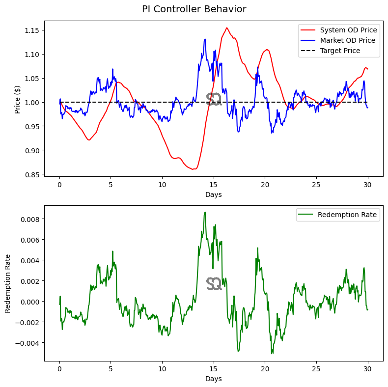
Figure 4.: Example of a PI Controller behavior
AMM Module
As the entire purpose of evaluating a stablecoin protocol relies on capably modeling whether the stablecoin’s market price retains its peg, it is crucial for the modeling effort to also simulate an exogenous liquidity pool which arbitrageurs and liquidators alike can use to access $OD liquidity. We model an abstract AMM whose liquidity distribution is derived by analyzing swap-in/swap-out curves extracted empirically by querying the 1inch aggregator on ETH-USDC swaps.
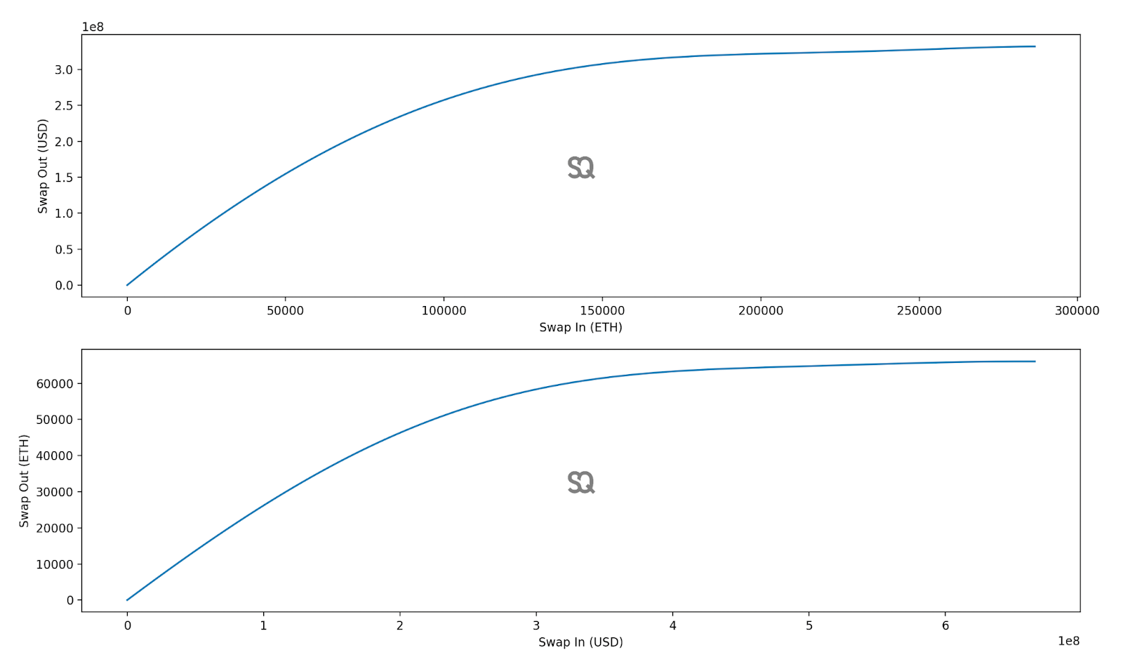
Figure 5.: Swap curves for ETH-USDC pair sampled from the 1inch aggregator
The curves can be rescaled by their maximum swap-out amounts (swap_out_max) and the smallest swap-in amount (swap_in_bar) that achieves this maximum swap-out amount. In doing so, we obtain a very natural description of the swap curves that is independent of the absolute amounts of funds actually held in the pools.
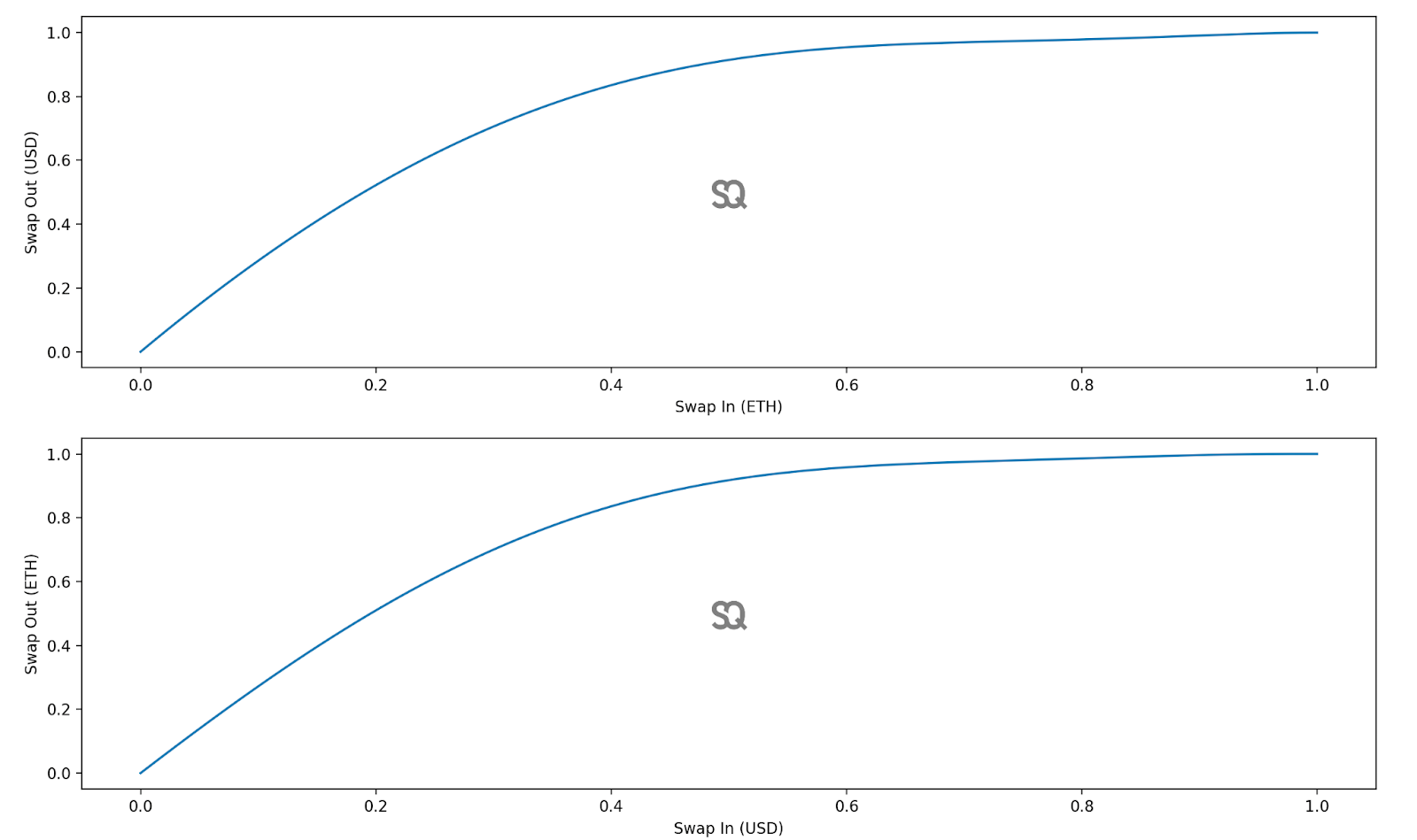
Figure 6.: Rescaled swap curves for ETH-USDC pair sampled from the 1inch aggregator
The rescaled swap curves encode the relative liquidity distribution of the AMM (more specifically, its derivative). We assume that the shape of the rescaled swap curves remains the same throughout the entire simulation and only the amount of liquidity consumed, and total liquidities deposited/withdrawn from the AMM are adjusted as a result of swapping and stake/unstake operations.
Even under the assumption of static relative liquidity, we can model very expressive slippage curve behavior as the pool is drained and rebalanced. As an example, we can model large drainages of the pool. Shown here are the resulting swap out curves after performing a large ETH->USD swap which drains 30% of the available USD liquidity:

Figure 7.: Swap curves for ETH-USDC pair after pool drainage
We can also straightforwardly model liquidity injections and removals from this abstract AMM. Shown below, we take the state of the AMM shown above (after the large ETH->USD swap was performed), and show what the state of the AMM becomes if an agent boosts the liquidity by 20%:

Figure 8.: Swap curves for ETH-USDC pair after adding liquidity
At any given moment, the AMM module allows us to query precise amounts required for performing arbitrage operations, as well as exactly solving for the optimal loan repayment amount which maximizes a liquidator’s profit (see Appendix B.1).
Hyperparameter optimization
Hyperparameter optimization plays a pivotal role in improving the accuracy and reliability of risk models. For our project, we utilized Bayesian optimization techniques to effectively explore the vast search space of potential PI Controller parameter sets. This approach focuses on refining the settings for the proportional (Kp) and integral (Ki) gains of the PI Controller.
Our chosen objective was to minimize the average maximum divergence between the market price and the target peg value of $1. Given the wide logarithmic range that Kp and Ki values can be chosen from, we apply the Tree-structured Parzen Estimator algorithm to aid in selecting the next parameter to investigate.
The findings and detailed discussion of the hyperparameter optimization process are presented in the “Results” section of this report, where we analyze the impact of various parameter settings on model performance and system stability.
Assumptions
Each modeling exercise is underpinned by a series of assumptions that simplify the complex realities of the system being studied. Some of the key assumptions used in our simulation are outlined below.
AMM Liquidity
We assume that the relative swap liquidity distribution (as defined through normalized swap-in/swap-out curves) remains static throughout the entire simulation with only the absolute liquidity amounts changing as a result of swap and stake/unstake operations.
User Behavior
Users in our simulation follow a simplistic behavioral model. They are not “intelligent” in the sense that their actions are governed by a set of predefined rules and probability distributions rather than by strategic decision-making aimed at optimizing their positions under current market conditions. They do not employ deliberate trading strategies, nor do they adjust their positions to strategically avoid liquidations or to maximize their leverage.
Arbitrage and Liquidations
Our model assumes that arbitrageurs and liquidators behave rationally, engaging with the protocol only when it is profitable to do so. While this assumption mirrors the behavior of sophisticated market participants, it might be overly optimistic as it assumes that all profitable opportunities are acted upon. To address potential criticisms that small profit margins might go unexploited, thus skewing the realism of our model, we have introduced a minimum profit threshold. This threshold must be exceeded for an arbitrage or liquidation action to occur. Adding this criterion did not qualitatively alter the outcomes of our simulations.
Results
PI Controller
We have utilized our hyperparameter optimization framework to begin refining the settings of the PI Controller, conducting ~10k experimental trials. These efforts aim to identify the most effective parameters to maintain the desired stability of the $OD price. The initial results of these extensive simulations are summarized below:

Figure 9.: Rank plot showing the relationship between the PI Controller parameters and the objective function
The accompanying chart provides a high-level perspective on these initial results, with both axes (Ki for the integral gain and Kp for the proportional gain) displayed on a logarithmic scale to capture a wide range of values. Each data point on the chart represents an individual trial characterized by a specific set of Kp and Ki values. The points are color-coded based on the normalized average objective value obtained across all simulation runs for those parameters, where the objective value is the error rate we are striving to minimize. Notably, two regions displaying clusters of data points with low objective values are enclosed in red squares. These clusters are critical as they indicate parameter sets that yielded the lowest error rates, suggesting they are particularly effective at stabilizing the $OD price.
Cluster A, suggests focusing on the following bounds
Kp:
- Lower Bound: -6 (log), 1e-6 (decimal)
- Upper Bound: -4 (log), 1e-4 (decimal)
Ki:
- Lower Bound: -16 (log), 1e-16 (decimal)
- Upper Bound: -14 (log), (1e-14) decimal
Cluster B, suggests focusing the following bounds
Kp:
- Lower Bound: -5.5 (log), 3.16e-6 (decimal)
- Upper Bound: -4.5 (log), 3.16e-5 (decimal)
Ki:
- Lower Bound: -12.5 (log), 3.16e-13 (decimal)
- Upper Bound: -11 (log), (1e-11) decimal
Subsequent charts break down the data further by separately analyzing the Kp and Ki parameters. These charts plot the parameters against their respective objective values and are color-coded by the number of simulation runs conducted with each parameter set.

Figure 10.: Kp parameter values against the resulting objective function value
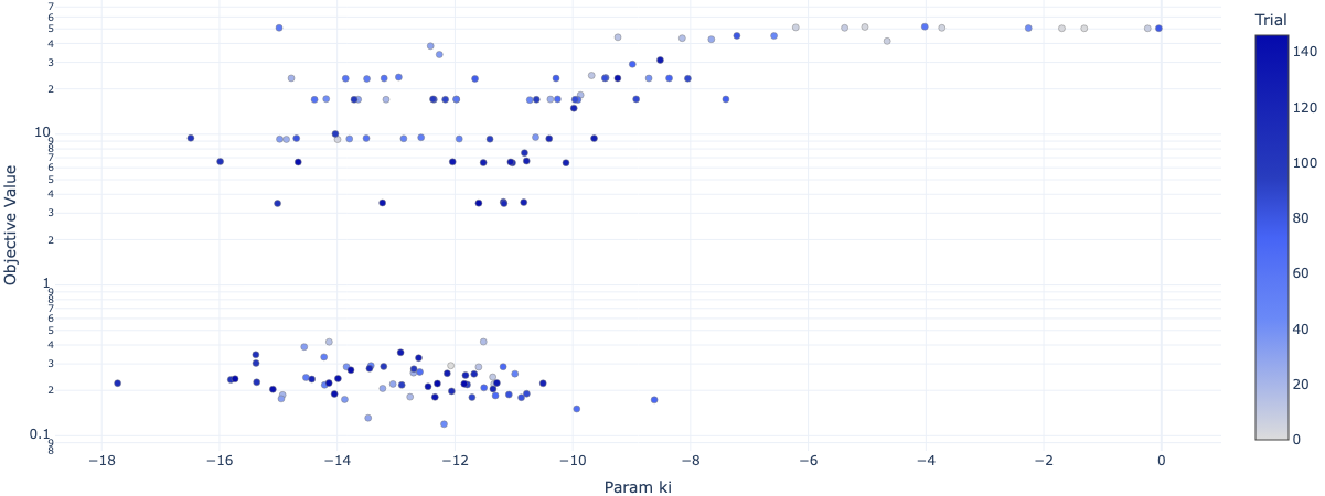
Figure 11.: Ki parameter values against the resulting objective function value
Consistent with the overarching trends observed in the comprehensive chart, these detailed plots also show clustering in the same regions. This consistency reinforces our confidence in these areas as focal points for further fine-tuning and optimization.
Collateral Factors
In the Open Dollar protocol, collateral factors (CFs) are pivotal in determining the borrowing limits against specific collateral assets. Expressed as a percentage, the CF indicates the amount of collateral needed to borrow a certain value; for example, a CF of 150% implies that to borrow $100, a user must deposit $150 in collateral.
Setting the appropriate CFs involves balancing two critical objectives: minimizing insolvency risk and maximizing capital efficiency.
- Capital Efficiency: A lower CF allows users to leverage their assets more effectively, increasing the capital efficiency of their investments.
- Insolvency Risk: Conversely, reducing the CF heightens the risk of insolvency for the protocol, particularly if sharp market price fluctuations cause positions to become undercollateralized. In severe cases, this could lead to significant bad debt, potentially jeopardizing the entire system.
To navigate these trade-offs, we conducted simulations across a spectrum of CFs to evaluate their impact on protocol stability and efficiency. The simulations measured two key metrics:
- Average Bad Debt Ratio: This metric reflects the average amount of bad debt as a percentage of the Total Value Locked (TVL) in the protocol.
- Undercollateralized User Ratio: This is the proportion of users whose positions become undercollateralized, relative to the total user base.
The chart below depicts the relationship between CF levels, the undercollateralized user ratio, and the bad debt ratio.

Figure 12.: Undercollateralization Frontier
As one can see, both of these values go hand-in-hand. Both the undercollateralized users ratio and the bad debt ratio remain flat until around 120% CF. More aggressive values introduce exponentially more insolvency risk to the protocol, while improving the users’ capital efficiency only linearly. 120% collateral factor should be the absolute minimum that the ETH LSTs should have in the Open Dollar protocol. This level optimally balances the risks of insolvency with the benefits of increased capital efficiency, ensuring both stability and operational viability for the protocol.
Stable Assets
The rationale behind selecting collateral factor (CF) parameters for LSTs involves a specialized form of risk assessment specifically tailored to stablecoin assets (LSTs, akin to ETH-stable assets). The risks associated with these assets cannot be modeled through simple price stress testing, as their primary risk lies structurally in their potential to depeg from their underlying asset.
For these assets, our focus is on determining the net depeg tolerance that the protocol can withstand. This calculation necessitates dynamic real-time updating, typically involving an analysis of both available decentralized exchange (DEX) liquidity and the utilization of these assets as collateral on other Arbitrum lending protocols. However, as a rough guideline, the difference between 100% and the sum of inverse of collateral factor and the liquidation incentive provides an approximate measure of the magnitude of a depeg event that risks rendering Open Dollar positions insolvent.
For Open Dollar stable assets, these depeg tolerances amount to 10-15%.
The primary depeg risk for rETH and wstETH arises from the potential slashing penalties incurred by their validators. Given the extensive validator sets offered by both decentralized autonomous organizations (DAOs), a significant portion of validators would need to be slashed over a course of multiple days for a substantial depeg event to occur.
This results in initial collateral factors of 130%, providing a balanced starting point.
Recommendations
PI Controller
When it comes to the final recommendation of which Kp and Ki params should be set at the protocol initialization, there is no single best framework. Ultimately, each set of parameters comes with its own tradeoffs. Choosing smaller parameters can lead to the PI Controller not being effective enough, resulting in long periods of time where the market or redemption prices diverge significantly from the target. Contrastingly, if the PI parameters are set too large, the system is likely to overcorrect given minor perturbations and become unstable in the long run. Furthermore, focusing the individual parameters that showed the best results in the protocol simulations could in principle have been just right to handle the randomness that drove the simulator on that specific simulation run (the opposite is also true). It is for this reason that we instead focus on regions where we see clusters of well-performing parameter values.
Currently, Reflexer’s RAI employs the following PI parameters:
- Kp: 1.11001102931e-07
- Ki: 3.2884e-14
The 0xSQ recommended parameters for Open Dollar are:
- Kp: 3.16e-6 (3160000000000 in WAD)
- Ki: 3.16e-13 (316000 in WAD)
As a sanity check, our results are roughly consistent, in magnitude, with these values.
Collateral Factors
In the light of results discussed in one of the previous sections, the recommended collateral factors are:
- wstETH: 130% (120% minimum)
- rETH: 130% (120% minimum)
Next steps / further research
As we continue our partnership with Open Dollar, 0xsidequest is committed to further enhancing and developing the protocol. We believe in the power of collaborative effort and community involvement in refining and expanding the capabilities of decentralized systems such as Open Dollar.
We encourage the wider community to participate in discussions about our methodologies and potential improvements. Community feedback is invaluable, and we believe that an engaged and active community is crucial to the iterative process of refining decentralized protocols. Whether you are a developer, a researcher, or simply an enthusiast in the DeFi space, your insights can make a significant impact.
Future research into the mechanics of Open Dollar could include:
- Introducing New Assets: Assessing additional collateral assets for integration into the protocol could provide new opportunities. This research would involve thorough testing and risk analysis to ensure compatibility with Open Dollar’s stability and security standards.
- Exploring PI Controller Update Delays: Investigating the impact of delays in updating the PI Controller could offer insights into optimizing protocol responsiveness. This area of research would aim to understand how such delays affect market reactivity and to formulate strategies to mitigate any negative impacts.
- Continuous Parameter Optimization: There is an ongoing need to refine the parameters controlling the protocol, such as those of the PI Controller. Research could focus on regularly updating and optimizing these parameters to better align with market dynamics and research outcomes. Furthermore, we stress the importance of exploring multiple other objective functions and collecting more datapoints on extreme stress scenarios.